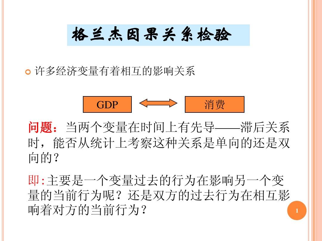
關係
(Granger Causality)
要探討因果關係,首先當然要定義什麼是因果關係。這裡不再談伽利略抑或
休謨等人在哲學意義上所說的因果關係,只從統計意義上介紹其定義。
從統計的角度,因果關係是通過機率或者分布函式的角度體現出來的:在宇宙中所有其它事件的發生情況固定不變的條件下,如果一個事件A的發生與不發生對於另一個事件B的發生的機率(如果通過事件定義了隨機變數那么也可以說分布函式)有影響,並且這兩個事件在時間上有先後順序(A前B後),那么我們便可以說A是B的原因。早期因果性是簡單通過機率來定義的,即如果P(B|A)>P(B)那么A就是B的原因(Suppes,1970);然而這種定義有兩大缺陷:一、沒有考慮時間先後順序;二、從P(B|A)>P(B)由條件機率公式馬上可以推出P(A|B)>P(A),顯然上面的定義就自相矛盾了(並且定義中的“>”毫無道理,換成“<”照樣講得通,後來通過改進,把定義中的“>”改為了不等號“≠”,其實按照同樣的推理,這樣定義一樣站不住腳)。
事實上,以上定義還有更大的缺陷,就是信息集的問題。嚴格講來,要真正確定因果關係,必須考慮到完整的信息集,也就是說,要得出“A是B的原因”這樣的結論,必須全面考慮宇宙中所有的事件,否則往往就會發生誤解。最明顯的例子就是若另有一個事件C,它是A和B的共同原因,考慮一個極端情況:若P(A|C)=1,P(B|C)=1,那么顯然有P(B|AC)=P(B|C),此時可以看出A事件是否發生與B事件已經沒有關係了。
因此,Granger於1967年提出了Granger因果關係的定義(均值和方差意義上的均值因果性)並在1980年發展將其進行了擴展(分布意義上的全民因果性),他的定義是建立在完整信息集以及發生時間先後順序基礎上的。
從便於理解的角度上按照從一般到特殊的順序講:
最一般的情況是根據分布函式(條件分布)判斷。約定
是到n期為止宇宙中的所有信息,
為到n期為止所有的
(t=1…n),
為第n+1期X的取值,
為除Y之外的所有信息。Y的發生影響X的發生的表達式為:
後來認為宇宙信息集是不可能找到的,於是退而求其次,找一個可獲取的信息集J來替代Ω:
再後來,大家又認為驗證分布函式是否相等實在是太複雜,於是再次退而求其次,只是驗證期望是否相等(這種叫做均值因果性,上面用分布函式驗證的因果關係叫全面因果性):
也有一種方法是驗證Y的出現是否能減小對
的預測誤差,即比較方差是否發生變化:
檢驗
(Granger Causality Test)
可以看出,我們所使用的Granger因果檢驗與其最初的定義已經偏離甚遠,削減了很多條件(並且由回歸分析方法和F檢驗的使用我們可以知道還增強了若干條件),這很可能會導致虛假的因果關係。因此,在使用這種方法時,務必檢查前提條件,使其儘量能夠滿足。此外,統計方法並非萬能的,評判一個對象,往往需要多種角度的觀察。正所謂“
兼聽則明,偏聽則暗”。誠然真相永遠只有一個,但是也要靠科學的探索方法。
英語翻譯
Granger causality test is a technique for determining whether one time series is useful in forecasting another.Ordinarily, regressions reflect "mere" correlations, but Clive Granger, who won a Nobel Prize in Economics, argued that there is an interpretation of a set of tests as revealing something about causality.
A time series X is said to Granger-cause Y if it can be shown, usually through a series of F-tests on lagged values of X (and with lagged values of Y also known), that those X values provide statistically significant information about future values of Y.
The test works by first doing a regression of Δ
Y on lagged values of Δ
Y. Once the appropriate lag interval for
Y is proved significant (t-stat or
p-value), subsequent regressions for lagged levels of Δ
X are performed and added to the regression provided that they 1) are significant in and of themselves and 2) add explanatory power to the model. This can be repeated for multiple Δ
Xs (with each Δ
X being tested independently of other Δ
Xs, but in conjunction with the proven lag level of Δ
Y). More than one lag level of a variable can be included in the final regression model, provided it is statistically significant and provides explanatory power.
The researcher is often looking for a clear story, such as X granger-causes Y but not the other way around. In practice, however results are often hard-to-interpret. For instance no variable granger-causes the other, or that each of the two variables granger-causes the second.
Despite its name, Granger causality does not imply true causality. If both X and Y are driven by a common third process with different lags, their measure of Granger causality could still be statistically significant. Yet, manipulation of one process would not change the other. Indeed, the Granger test is designed to handle pairs of variables, and may produce misleading results when the true relationship involves three or more variables. A similar test involving more variables can be applied with vector autoregression. A new method for Granger causality that is not sensitive to the normal distribution of the error term has been developed by Hacker and Hatemi-J (2006). This new method is especially useful in financial economics since many financial variables are non-normal.
This technique has been adapted to neural science..
Here is an example of the function grangertest() in the lmtest library of the
R package:
Granger causality test
Model 1: fii ~ Lags(fii, 1:5) + Lags(rM, 1:5)
Model 2: fii ~ Lags(fii, 1:5)
Res.Df Df F Pr(>F)
1 629
2 634 5 2.5115 0.02896 *
---
Signif. codes: 0 '***' 0.001 '**' 0.01 '*' 0.05 '.' 0.1 ' ' 1
Granger causality test
Model 1: rM ~ Lags(rM, 1:5) + Lags(fii, 1:5)
Model 2: rM ~ Lags(rM, 1:5)
Res.Df Df F Pr(>F)
1 629
2 634 5 1.1804 0.3172
The first Model 1 tests whether it is okay to remove lagged rM from the regression explaining FII using lagged FII. It is not (p = 0.02896). The second pair of Model 1 and Model 2 finds that it is possible to remove the lagged FII from the model explaining rM using lagged rM. From this, we conclude that rM granger-causes FII but not the other way around.


